ai-toolbox
deep dive into applications and algorithms
Sliding Detection for Friction Welding Machine Tools Using AI
Real‑time AI monitoring to detect workpiece slippage in friction welding.
 Production Data
Testing Data
Production Data
Testing Data
Raw Data - Training
The data is obtained from the friction welding machine’s control PLC through the MQTT protocol. The PLC Siemens 1500 includes a program that sends JSON messages containing the data values and timestamp to a Mosquitto broker installed on a Linux server. On the same server, a service implemented in Python reads these messages and generates CSV files that store all the collected data. To implement the real‑time detection system, another similar service is used, which periodically calls the detection function with a window of the most recent data, at a configurable time interval.
Two distinct Designs of Experiments (DOEs) were carried out, resulting in the production of 81 welds with a diameter of 20 mm and 20 welds with a diameter of 40 mm. For each diameter, half of the welds were manufactured under standard production conditions, while the remaining half were intentionally produced with an induced defect in order to generate a sliding phenomenon. In the welds with induced defects, two different behaviors were observed: in some cases, the welding process had to be interrupted due to excessive sliding, whereas in others the process was able to reach completion despite the sliding presence.
Using the developed platform, the following variables are monitored: Timestamp, Spindle Torque (Nm), Spindle Speed (rpm), Slide Force (kN), Slide Position (mm), Step, Spindle Clamp Pressure (bar), Spindle Clamp Position (mm), Slide Clamp Pressure (bar) and Slide Clamp Position (mm). As the output variable, a binary label is recorded to indicate whether the sliding phenomenon occurred during each welding cycle. This label constitutes the ground truth for the subsequent analysis and model development. It is important to note that, although the label confirms the presence or absence of sliding, the exact timestamp at which the sliding phenomenon occurs within the time series is not available.
Learn moreRaw Data - Testing/Production
Preprocessing - Training Data
Once we have examined the ranges, structure, and patterns of each variable as part of the descriptive analysis, we proceed to analyze the linear correlations between them. In both correlation plots, we can confirm what we observed previously: our label is highly correlated with two specific variables whose values differ clearly between slicing and non‑slicing cases.
However, we do not want the model to learn from these lower absolute values; instead, our goal is for the model to learn from the underlying temporal patterns. Therefore, we will apply a preprocessing stage to these time series with the goal of removing the influence of absolute values and focusing exclusively on the dynamic patterns of the signals. This preprocessing includes two key steps: signal smoothing and signal normalization.
First, smoothing allows us to reduce high‑frequency noise present in the raw measurements, making it easier to identify the true underlying trends of the welding process. Techniques such as moving averages, Savitzky–Golay filters can help highlight the general shape of the signal without distorting it.
Second, we will apply normalization to make the signals comparable across different welds and to prevent the machine learning model from relying on anomalously low or high magnitudes. Min–max normalization or standardization (z‑score) have been used.
With this preprocessing, our goal is for the model to learn the relevant temporal characteristics—how the signal evolves over time, its changes, peaks, and transitions—rather than the differences in absolute magnitudes that we already know distinguish slicing from non-slicing cases. This will lead to a more robust and generalizable model.
Learn morePreprocessing - Testing/Production Data
Dataset - Training
The training dataset is composed of multivariate time‑series signals recorded during friction welding operations, including torque, pressure, and force measurements. To enable the use of traditional machine learning models on each individual weld, these raw signals are transformed into compact feature vectors by extracting descriptive statistical features—specifically the mean, standard deviation, minimum, and maximum of each time series. This process summarizes the global behavior of the weld while reducing dimensionality. After feature extraction, the dataset is normalized using a MinMax Scaler, preparing it for robust model training. Given the limited number of samples, particularly for the 40 mm diameter group, the dataset is evaluated using Leave‑One‑Out Cross‑Validation (LOOCV), which allows us to assess model performance by iteratively training on all welds except one and testing on the remaining instance.
Learn moreDataset - Testing/Production
Learn moreModel Training
The model training followed two complementary approaches. First, statistical features were extracted from each weld and used to train a Random Forest classifier. To ensure robust evaluation with the limited dataset, Leave‑One‑Out Cross‑Validation (LOOCV) was applied. All features were scaled using a MinMax Scaler before training.
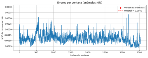
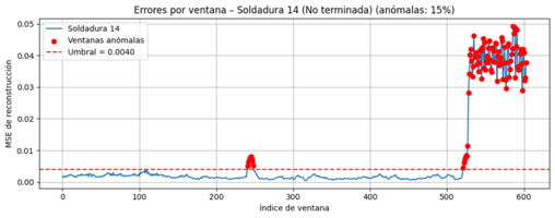
In the second approach, an LSTM Autoencoder was used to detect where slicing occurs within the weld. All weld signals were concatenated, and sliding windows were created to preserve temporal structure. The Autoencoder was trained exclusively on non‑slicing welds to learn normal behavior. During testing, reconstruction errors were used to identify abnormal windows, allowing precise localization of the slicing phenomenon within the welding process.
Learn moreTrained Model
The trained model consists of two complementary components. First, a Random Forest classifier was developed using statistical features extracted from each weld. The features were normalized using a MinMax Scaler, and the model was trained through Leave‑One‑Out Cross‑Validation to ensure robustness with the limited dataset. A second model, an LSTM Autoencoder, was trained exclusively on non‑slicing welds to learn the normal temporal patterns of the welding process.
Learn moreModel Testing
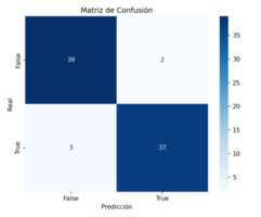
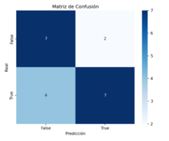
The Random Forest model was tested iteratively through LOOCV, evaluating its performance separately for 20 mm and 40 mm weld diameters. Confusion matrices, accuracy, and weighted F1 scores were used to quantify classification performance. For the LSTM Autoencoder, testing involved computing the reconstruction error on sliding windows generated from both good and defective welds. Windows with abnormally high errors were identified as indicators of slicing.
Learn moreTested Model
The final model combines global weld‑level classification with localized anomaly detection. The Random Forest provides a reliable binary decision for 20 mm welds, while the LSTM Autoencoder enables temporal localization of slicing events within the process. Together, they form a robust solution capable of both detecting the presence of sliding and identifying the specific regions where it occurs.
Learn moreMotivation
This experiment represents a step forward in bringing intelligence and autonomy to friction welding machine tools. By exploring AI‑powered sliding detection during the welding process, we aim not only to enhance operator awareness but also to introduce a lightweight and agile solution that can be deployed directly onto existing machine hardware. Leveraging real data from BERKOA’s IoT‑enabled test bench, we will transform raw torque, pressure, and force readings into meaningful insights that reveal hidden patterns behind the sliding phenomenon. This effort lays the foundation for future adaptive, self‑optimizing controllers capable of learning from every weld cycle. Beyond improving quality control and reducing maintenance needs, this project sparks innovation by applying AI to mechanical behaviours that were previously difficult to quantify. Ultimately, Sliding Detection is more than an experiment—it is a strategic step toward smarter machines, more efficient production, and a more advanced technological portfolio for the future.
Objective
This experiment, Sliding Detection for Friction Welding Machine Tools Using AI, aims to explore the feasibility of developing an AI-powered algorithm to detect workpiece slippage during the friction welding process. The goal is to provide feedback to the operator, with a solution that is lightweight and agile enough to be deployed on existing machine hardware. In the long term, this experiment will contribute to the development of predictive, self-optimizing adaptive controllers, enriching our portfolio with more mature and intelligent solutions. We anticipate several benefits from this project:
- Enhanced Quality Control: AI-driven insights will help detect anomalies and ensure consistent quality in our products.
- Reduced Maintenance: Predictive maintenance can be implemented based on the data analysis, reducing downtime and extending equipment lifespan.
- Innovation: The use of AI in analysing mechanical phenomena can lead to new insights and innovations in welding technology.
Use of AI
SLIDE application idea involves leveraging an existing IoT platform on a test bench machine in BERKOA facilities to extract and analyse data from the controller, focusing on parameters such as torque, pressure, and forces. This data will be used to conduct experiments on welding machine jigs, specifically to study and detect the sliding phenomenon (unwanted movement of workpiece mounted in static clamp) during the welding process.
AI technology will be used primarily in the following areas:
- Data Analysis: To process the vast amounts of data collected from the the controller and identify patterns related to the sliding phenomenon.
- Real-time Monitoring: To provide detailed, specific and real-time insights from the welding process, allowing -in future- for immediate adjustments to optimize performance.
Service reciever company
Berkoa S.C.O.O.P
https://www.berkoa.com/en/berkoa-s-coop/Description
Berkoa, S.Coop. is a tool manufacturing company. It is located in Elgoibar (Gipuzkoa), in the heart of the Basque Country, where there is a strong tradition of machine tool manufacturing.
Company offering
- Tool Machining

Service provider company
LORTEK
https://www.lortek.esDescription
LORTEK is a non-profit private technology centre that advances the digitalisation of manufacturing processes and transfers knowledge to industry, boosting competitiveness and sustainability. With a vision to lead in digital and smart manufacturing, LORTEK develops innovative solutions to address the challenges of digital transformation and the energy-climate transition.
Company service
- Process monitoring and control AI Services
Project Results
- 30% reduction in manual inspection time
- 15–20% decrease in scrap and rework, and
- a payback period of approximately two years, supported by reduced waste and increased product quality.
The model shows strong performance for the 20 mm weld diameter, achieving an accuracy of 0.94 and a weighted F1 score of 0.94, with the confusion matrix indicating only a few misclassifications. This confirms that the classifier generalizes well and reliably distinguishes slicing from non‑slicing cases for this diameter. In contrast, performance drops for the 40 mm diameter, where both accuracy and weighted F1 score reach 0.70. The higher number of misclassifications reflects the limited and more variable nature of this subset, making the classification task more challenging.
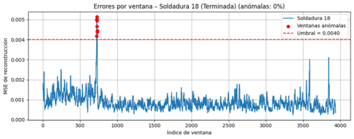
The LSTM Autoencoder also demonstrates solid performance, achieving an overall detection rate of 85% (34/40). For welds completed successfully, detection reaches 75% (15/20), while for severely affected welds that fail due to slicing, performance rises to 95% (19/20). Additional false‑positive testing on eleven independent good welds shows that only one weld slightly exceeded the anomaly threshold, confirming a low false‑positive rate and stable detection of normal behavior.
Several key achievements stand out from the project. First, the statistical‑feature‑based Random Forest model successfully classifies slicing for the 20 mm diameter with high reliability, demonstrating that simple descriptive features capture the defect signature effectively. Second, the development of the LSTM Autoencoder provides not only accurate detection of the slicing phenomenon but also precise localization of where it occurs within the weld thanks to the window‑based reconstruction‑error analysis.
Additionally, the model shows robustness against false positives, correctly identifying stable welding processes in nearly all independent normal welds. Overall, the project delivers a combined classification‑and‑detection framework capable of identifying slicing, understanding when it emerges in the process, and providing a strong foundation for future real‑time monitoring and adaptive control solutions.
Data
Raw Data
Raw data collection
The data used in this project is obtained directly from the friction welding machine’s control PLC through the MQTT protocol. The Siemens 1500 PLC publishes JSON messages containing the timestamp and the corresponding signal values to a Mosquitto broker installed on a Linux server. A Python service running on this server subscribes to the MQTT topics, reads the incoming messages in real time, and stores them in CSV files, thus generating a structured record of all welding operations. To support the real‑time version of the detection system, a second Python service is used, which periodically requests the most recent data window at a configurable interval and sends it to the detection function.
Raw data description
For model development, two separate Design of Experiments (DOEs) were conducted to obtain training and testing data. A total of 81 welds were produced for the 20 mm diameter and 20 welds for the 40 mm diameter. For each diameter, half of the welds were manufactured under normal production conditions, and the other half were intentionally produced with an induced defect to generate the sliding phenomenon. Among the defective welds, two types of behavior were observed: some welds had to be stopped prematurely due to excessive sliding, while others were able to complete the process despite the defect.
The data acquisition platform records several process variables during each welding cycle, including Timestamp, Spindle Torque (Nm), Spindle Speed (rpm), Slide Force (kN), Slide Position (mm), Step, Spindle Clamp Pressure (bar), Spindle Clamp Position (mm), Slide Clamp Pressure (bar), and Slide Clamp Position (mm). Each weld is assigned a binary label indicating whether sliding occurred. This label serves as the ground truth for training and evaluating the machine learning models; however, it specifies only the presence or absence of sliding, not the exact time at which it begins within the time series.
Additionally, a separate validation dataset was collected to independently assess the robustness of the models. This second DOE consists of 30 additional welds of 20 mm diameter, of which 25 exhibit sliding and 5 are normal. These welds were not used during model training and provide an external reference to evaluate false positives, generalization, and real operating conditions.
Data preprocessing
Processing description
The raw multivariate time‑series signals were cleaned, synchronized, and segmented. For the classification task, each weld was aggregated into statistical summaries. For the anomaly‑detection task, the full sequences were concatenated and divided into overlapping sliding windows to preserve temporal structure.
Feature engineering
For each signal, descriptive statistical features were computed: mean, standard deviation, minimum, and maximum. These engineered features compress the full time series into compact vectors suitable for traditional machine‑learning models.
Algorithms
MinMaxScaler
Rescales each feature to a specified range, or [0, 1] by default, to prevent any variable from dominating the model and ensure consistent numerical behavior.
Features
Multi-dimensional time serie
An ensemble of N dimensional values indexed over time.
Raw Data
Data preprocessing
Datasets
Friction Welding Dataset – DOE 1 (Training & Validation)
License:
Internal / Proprietary
Size
101 welds total (81 welds of 20 mm, 20 welds of 40 mm), stored as CSV time series
This dataset contains raw process signals collected from the friction welding machine’s PLC, captured via MQTT and stored as CSV logs. Each weld includes multiple synchronized time‑series variables—torque, spindle speed, forces, positions, clamp pressures, and timestamps—along with a binary label indicating the presence or absence of sliding. The dataset contains balanced examples for each diameter, including both normal welds and welds with intentionally induced slicing defects.
In the following plots, we can observe the values of each variable throughout the welding process. The red curves correspond to welds in which the slicing phenomenon was intentionally induced, while the blue curves represent welds carried out under normal conditions, such as those with diameters of 20 mm and 40 mm.
Friction Welding Dataset – DOE 2 (Independent Validation)
License:
Internal / Proprietary
Size
30 welds total (20 mm diameter: 25 slicing, 5 non‑slicing), stored as CSV time series
This dataset contains raw process signals collected from the friction welding machine’s PLC, captured via MQTT and stored as CSV logs. Each weld includes multiple synchronized time‑series variables—torque, spindle speed, forces, positions, clamp pressures, and timestamps—along with a binary label indicating the presence or absence of sliding. The dataset contains balanced examples for each diameter, including both normal welds and welds with intentionally induced slicing defects.
In the following plots, we can observe the values of each variable throughout the welding process. The red curves correspond to welds in which the slicing phenomenon was intentionally induced, while the blue curves represent welds carried out under normal conditions, such as those with diameters of 20 mm and 40 mm.
Trained model/s
Model types
Model selection
- Robust to nonlinear relationships and feature interactions across signals.
- Performs well with tabular, low‑dimensional statistical features (mean, std, min, max).
- Provides stable results with limited data and avoids heavy hyperparameter tuning.
Hardware used for training
- Training was performed locally on a Windows workstation using CPU only, with no GPU acceleration required.
- Requirements: Python 3.11, scikit‑learn.
Model training
- Inputs: per‑weld feature vectors (mean, std, min, max for each signal), MinMax‑scaled.
- Validation: Leave‑One‑Out Cross‑Validation (LOOCV).
- Trained separately by diameter (20 mm and 40 mm) to reflect process geometry differences.
Loss function
- Not explicitly optimized via a differentiable loss.
Model testing
- LOOCV predictions aggregated to compute metrics and produce confusion matrices.
- Results reported separately for 20 mm and 40 mm welds.
Testing metrics
- Accuracy
- Weighted F1
- Confusion Matrix
Tested model
- 20 mm diameter: Accuracy 0.94, Weighted F1 0.94; few misclassifications; high reliability.
- 40 mm diameter: Accuracy 0.70, Weighted F1 0.70; performance limited by data volume/variability.
- Inference time: milliseconds per weld (CPU).
- Model size: small.
License:
Unknown
Figures
Figures
Model selection
- Captures temporal dependencies in multivariate signals.
- Trained on normal (non‑slicing) behavior to learn typical dynamics; anomalies (sliding) produce higher reconstruction error.
- Enables localization in time via windowed reconstruction error.
Hardware used for training
- Training was performed locally on a Windows workstation using CPU only, with no GPU acceleration required.
- Requirements: Python 3.11, deep learning framework (TensorFlow); training time minutes depending on windowing and epochs.
Model training
- Preprocessing: concatenate welds, create overlapping sliding windows to preserve temporal structure; MinMax scaling applied.
- Training data: only non‑slicing weld windows.
Objective: minimize reconstruction error (input vs. output) to model normality. A threshold on reconstruction error is selected
Loss function
- Reconstruction loss (e.g., Mean Squared Error) over multivariate windows.
Model testing
- Evaluate reconstruction error on windows from both good and defective welds.
- Flag windows exceeding the threshold as anomalous; aggregate at weld level (presence/absence) and visualize time‑localized detections.
- Additional independent validation on 30 welds (20 mm): 25 slicing and 5 non‑slicing.
Testing metrics
- Detection rate (overall and stratified by weld outcome).
Tested model
- Overall detection: 85% (34/40).
- Completed welds: 75% (15/20) detection.
- Failed due to slicing: 95% (19/20) detection.
- Independent good-weld subset: low false positives (only 1/11 slightly above threshold).
- Inference: near‑real‑time via periodic windows (configurable interval).
License:
Unknown
Figures
Figures